Modeling Life Effectively Disproves Zombies

Zombies are on fire right now. From Zombie Nation to Zombieland, it's clear that our culture has fully embraced the concept of mindless drones living among everyday citizens. Thanks (no thanks) to the Twilight series for the assist in making the whole monsters in society thing acceptable (to high school girls; whose boyfriends are dragged along to the movie and have to suffer through listening to every other girl drool over the meth'ed up characters in that story).

To this trend I say, NO! I'm calling shenanigans on zombies. Here's why:

What is a zombie? Is it a virus? Dawn of the Dead, the 28 Days Laters, I am Legend, etc. would suggest that it is. We'll go ahead and say yes. There are plenty of models that predict dispersion patterns of viruses in society, but we can work at an even more basic level than this.

Is a zombie still a human? Dawn of the Dead: No. Shawn of the Dead: Yes - AND you can play video games with them. Essentially, zombies are known as the "living dead," so I'll begin modeling from here to highlight the two main physical differences between humans and zombies.

Humans are inefficient machines. We emit about 150 watts of energy as overall body heat. Although it would be more efficient to be cold blooded, we found certain advantages to remaining mobile and having an active metabolism when it gets cold. Further, the brain functions by sending around 20-40 watts of electrical signals around itself and throughout the rest of the body. When a zombie bites, a victim's body temperature drops and organs begin to fail. Other than the whole craving brains/flesh thing, the life of the human ends, thus the following model is developed:

The life model disprove zombies

Translated: A life is equal to a the sum of all days where the energy of ones body approaches 150 watts, and the energy of said brain approaches 20 watts. This is valid from a person's birth day to the n^th day of an individual's life, otherwise known as a "life span" (L_s - see below):

A life span is limited to n days

Thus, it is impossible for a being to operate once a brain ceases to function due to a lack of energy production of its carrying body. This goes for "infected" humans or other animals. There is probably a better metric of brain activity that I could use, but I figure this model gets the point across.

This is most importantly applicable when faced with a "I don't have time to zombify this costume" situation.

Office 2007, you're pushing my buttons! / Micosoft Inefficiency .NET

This is unacceptable! A mail client should not use the same amount of resources as GIS software. I am convinced that Outlook 2007 is making my other programs crash. I've said it before, and I'll say it again. Office 2007 missed the mark.

Here is a screenshot of my ArcMap editing session:


I am running Windows Media Player in the background with with 200+ songs on the playlist (topping out around 20,000 k of memory usage). I am assuming WMP references the songs via a list rather than caching all the 855 MB of files, however my media player is using fewer resources than my mail client is using.

Outlook is hogging just short of the almost 200,000 k that ArcMap uses - and it's just sitting there:

Rather than trying to make Office and Windows look like a Mac, why doesn't Microsoft take what they already have a make it more efficient? After that, go ahead and add the neat little trinkets (about which I honestly couldn't care less). There is absolutely no reason for my mail client to use such vast amounts of memory and processing power to sit there and ding a few dozen times a day.

Personal computer technology continues to increase at a terrific rate, and the price of powerful and small computers is steadily decreasing. The average user (non-tech/home computer user) seems to be utilizing web-based resources more and more. Other than gaming, I can only think of a few other examples of power users who need very elite computers: photo/graphics editors and video editors.

Taking advantage of this by writing software that runs efficiently would allow one to use a computer for more than a few years without it being bogged down (I'm looking at you, Windows XP). It takes my laptop a few minutes to open Mozilla. MINUTES! That is just stupid.

Instead, Microsoft continues to write clunky software that needlessly hogs computing resources so when the computer seems to become "out of date" in a year or two, unknowing consumers will go out and buy another laptop with a new and even more inefficient version of Windows products. This seems like planned obsolesence. Lame.

Well, I'm glad to see that Dell (and others I'm sure) is giving the option for new computers to be loaded with the free Ubuntu (Linux) OS. I've been meaning to give Linux a try. Even worse, another option is to "downgrade to Windows XP" on new systems. Fail.

Intro to Customizing ArcGIS Desktop, Toolbars, and Normal.mxt

While attempting to build a (forthcoming) custom tool for my ArcGIS environment, I encountered a problem: I cannot save my new custom toolbar to Normal.mxt. Every time I close and re-open ArcMap, the toolbar does not return.

I am attempting to construct a toolbar to use in my default environment, so naturally I begin working in a blank (Untitled) .mxd document. This is probably a problem: it seems that Normal.mxt is updated when the .mxd is saved or closed, so I'll start by creating a local project so the "save" command can be called.

The following is my version of a walkthrough that discusses how to properly add a toolbar to the Normal.mxt template.

• Start ArcMap with a new/blank document
• Save this document anywhere - location is not important. It can be deleted later. Again, I'm assuming that a saved document allows the .mxt file to be saved, thus edits can be applied, though this is just a hypothesis.
  
• Open the Customize dialog (from Tools :: Customize, or double click in a gray area beside a docked toolbar)

• Choose New to create a new, blank toolbar
• Give the new toolbar a name, and be sure to change the "Save in" option to Normal.mxt.
  ( Normal.mxt is the default, base template that ArcMap uses to define the which toolbars are included in its operating interface. When a new/blank document is launched, Normal.mxt is called to define which buttons and toolbars go where. Over time it is nice to change this around to suit individual needs)
  

• The new, blank toolbar is added to the project

• Add some buttons/tools/commands to the toolbar by navigating to the Commands tab from the Customize dialog. There are many provided by ESRI, sorted into Categories (the pane on the left) and the actual commands (buttons) are located in the Commands list to the right. Select the one you want and drag it carefully to the new toolbar, or to any other toolbar. Again, be sure to "Save in" Normal.mxt

• To add customized buttons from which you can run your own Visual Basic code, scroll all the way to the bottom of the Categories list and select [UIControls].
• Press the New UIControl... button
• Choose from one of the control types - UIButtonControl will make a button that will run some code that will be programmed later - and press Create
• Rename the control to something that will be recognized easily, and drag the control to the new toolbar
• Change the button's icon/picture by right clicking on the button (with the Customize dialog still launched) and choose an icon from the "Change Button Image" sub-menu.A custom .bmp file can be used as the image by choosing Browse from this menu

• To begin editing code, right click on a button (command) and choose View Source to launch the Visual Basic Editor (shortcut key Alt+F11)

• Now close the Customize dialog box and save the otherwise blank ArcMap document. From here the new toolbar and its tools should be saved in Normal.mxt.

• Just for the sake of argument, drag the toolbar to the top of the ArcMap window to dock it. (This really shouldn't be necessary though.)
  
  
• Save the document again
  
• Open the Customize dialog again and change the "Save in" option from Normal.mxt to the alternative choice which will be the name of the .mxd. If the toolbar is still present, the Normal.mxt template has been successfully altered with the addition of the new toolbar. Change the "Save in" option back to Normal.mxt and continue alterations if necessary.
  

See also:
ESRI Article: Save Custom Toolbar Configuration
My Normal.mxt

Languages of Modeling

I recently became interested in modeling everyday occurrences. This is mostly a joke, though it's definitely good practice to keep statistical analysis techniques fresh in my head. Additionally, it's helping me brush up on some much needed math topics that are in dire need of refreshment.

To effectively convey this information (nerdy jokes), I realize that I draw upon four sorts of languages: English, stats, math, and the newest L^AT_EX.

• English is used to concisely describe a situation: "Shaquille O'Neal is the greatest living actor"
• Statistical modeling is used to describe and quantify predictions, interactions, and tendencies: "My love of killing hookers by playing Grand Theft Auto is directly proportional to your love of killing literature by obsessing over Twilight - as modeled in relation to characters who look like they're addicted to meth." English is used as the core language, however the subset dialect of statistics is well defined. Certain graphs and diagrams are often added to convey an idea
• Mathematics are used to explicitly define what is happening in a specific, overly technical, dry-witted manor:

• and finally, the newest of which, L^AT_EX, is used to create the pretty looking mathematical and statistical functions and algorithms: (see above)

Throw in some HTML as the medium of dissemination, and you have one nerdy kid that needs to record more music and make some bad decisions.

LaTeX is a markup language used in typesetting information into standard, pre-existing document templates. Whereas writing a paper usually consists of typing text into MS Word and setting the page margins, paragraph spacing, indentations, etc., the same plain text of the paper can be pasted into the LaTeX environment with bits of markup wrapping around it. All standard formatting is automatically applied so numerious authors can easily produce articles with the same formatting.

Additionally, high quality formulas are easier to create. The methodical and intuitive prasing can get cluttered, but pretty much everything is grouped by braces ( { } ).

As an example, here is the code used to create the formula above:

Nickelback = {\sum{StabWounds}^{MyEars} \over{time}} - Enjoyment(life)

While reading just a little bit about it, I immediately began to recognize this as the formatting used in many of the journal articles that I read. Of course I learn about this on my way OUT of grad school! Instead I'll use it for nerdy internet jokes. Wonderful.

App Idea: Facebook History

I've tried on a few different occasions to see how I have previously wasted my time in the past. I scroll to the bottom of my Facebook wall, click "Older Posts" and repeat. This happens up to a half dozen times before I loose interest (I've read studies that internet users' attention span is as short as seven seconds [I would have posted links, but I don't feel like reading these articles]). This technique usually yields no more than a day or two of my Facebook history. Who cares?

I'd like a more efficient way to (possibly) quantify and (more importantly [not importantly]) reflect on just how much of my youth I have wasted. Assume each wall post can equal 10-20 seconds, each posted picture/link amounts to a bit more time, etc. Also, it'll just serve as a simple tool to navigate through a given time frame to see what you/your friends were up to at least 100 years ago.

Calculate Lat/Long Values in ArcMap

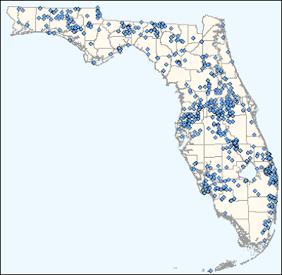
Yet again, I had a difficult time finding sufficient information on calculating latitude and longitude values for a point shapefile. I've only encountered one or two situations in the past few years where I worked with a coverage that was missing these data, though it's still a basic and important technique that should be addressed a bit better.

It turns out that (at least) ArcMap 9.2 provides a pretty simple method to quickly calculate a number of geographic coordinates. A few things are important to consider though:

Converting Polygon to Point data:
Unless you're interested in the locations of polygon boundaries (shorelines, property boundaries, etc. - in which case you will convert the polygon boundaries to nodes), you will want to create a point coverage to represent centroids. Be sure to choose whether that center location will be the true center, or be preserved within the bounds of the polygon:

• Show ArcToolbox in ArcMap (or ArcCatalog)
• Open the Feature to Point tool
  (Under Data Management Tools :: Features :: Feature to Point)
• Press Show Help to read more about the tool
• Select a polygon or line feature to use as in input featre
• Set an output location and name for the resulting feature class
• Check the "Inside" check box to calculate a centroid within the boundary of a given feature (i.e. a "bent" polygon similar to the shape of Florida can have a centroid in the Gulf of Mexico if "Inside" is not selected)
  

There is insufficient information on the internets about this process works. There is a simple and automated calculator built into atribute table field calculations. To make this work properly in this situation (calculating geographic latitude/longitude coordinates) the coordinate system must be set to a geographic coordinate system, rather than a projected coordinate system.

Calculating Lat/Long Coordinates:

• Add a point coverage to a project
• Change the data frame to a geographic coordinate system
  
  • Right click on the data frame heading in the table of contents pane and choose Properties
    
  • Navigate to the Coordinate System tab
  • Expand the Predefined branch
  • Expand the Geographic Coordinate Systems branch
  • Expand the North America branch
    
  • Choose North American 1983 HARN and click OK
  • Choose Yes if prompted with a coordinate system warning
    
• Open the layer's Attribute Table and add the following fields /types (LONG_DD is indeed string 3, not a typo)
  

Field Name LATITUDE LONGITUDE LAT_DD LAT_MM LAT_SS LONG_DD LONG_MM LONG_SS DATUM

Type/Length Text (string), 20 Text, 20 Text, 2 Text, 2 Text, 9 Text, 3 Text, 2 Text, 9 Text, 25

• Go ahead and calculate "North American 1983 HARN" (or whatever coordinate system you used) in the DATUM field.  Whomever uses this data in the future will need to the method used to calculate the units
• Now begin to calculate the units.  Right click the LATITUDE field and select Calculate Geometry
• Set the Property to "Select Y Coordinate of Point" (Latitude = y, and Longitude = x)

! Note that Latitude = y and Longitude = x. Usually you'll ask for "x/y coordinates" in geometry class, however surveyors ask for "a northing and an easting" - which flips the order of the x and y values around.

• Select "Use coordinate system of the data frame" to use the geographic coordinate system. After this, the Units will change from various length units of measure (meters, feet, etc.) to a number of DMS choices
• Select "Packed DMS Format (+/- DDD.MMSSssssss")" and hit OK
  
• Repeat this for LONGITUDE with "Select X Coordinate of Point"
• Use the Field Calculator to populate the remaining fields using the following formulas
• LAT_DD: left([LATITUDE], 2)
• LAT_MM: mid([LATITUDE], 4, 2)
• LAT_SS: right([LATITUDE], 8)/1000000
• LONG_DD: left([LONGITUDE], 3)
  
• LONG_MM: mid([LONGITUDE], 5, 2)
• LONG_SS: right([LONGITUDE], 8)/1000000
  

• Finally, be sure to Calculate Geometry again on the LATITUDE and LONGITUDE fields (Using the coordinate system of the data frame) but set the units to Decimal Degrees.  Until this is finished, the values look like decimal degrees, but if these coordinates are projected, they will be incorrect - perhaps by a long way.  A good trick is to see if any values after the decimal are greater than x.599999.  If there are any values between x.6 and x.9, those are indeed decimal degrees.

There are a few other formats that may be more appropriate for individual projects. Some custom utilities will require lat/long processing fields to match, so be careful with the LAT_DD/LONG_DD fields; thus DMS fields may need to be converted to another data type.  Further, field types of Double and Short Integer may be more appropriate for your database.

See also:
Angular Unit Conversion (convert between DD, DMS, and radians)
How To: Populate x, y, or z point data fields of an attribute table

How To: Calculate Latitude and Longitude values using the Field Calculator