Tuesday, April 28, 2009

Geostatistical Modeling of Surface Water Sediment Analytes

Presented April 27th, 2009 for Advanced Quantatitave Geography, Florida State University.

Introduction:

DEP Watershed Monitoring program holds a wealth of sampled water and sediment chemistry data. One particular analyte, Cadmium (Cd), is a toxic metal that is found naturally in soil, however it is also a component used in automobile brake pads. An exploratory investigation was attmempted, with the intentions of correlating lake and stream sediment-laden cadmium levels with population density. After numerous failed attempts of importing this dataset into R and GeoDa, this preliminary review of spatial autocorrelation is abandoned and alternative chosen. The new investigation will attempt to examine the spatial distribution of cadmium levels across the state of Florida.

Examination:
  • Plot the raw data
  • Plot the emperical variogram
  • Develop a reasonable variogram model
  • Use model together with the data to create a surface
  • Examine model diagnostics

Default kriging interpolation:

[Basic kriging geostatistical interpolation]


[Same surface with station location distribution]

This simple surface does a moderatly decent job of modeling the phosphate belt in west central Florida, extending east of Hillsborough County, as well as similar areas of phosphate mines around the big bend.


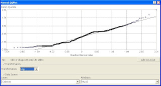
Check for dataset normality:

The histogram shows significant skewness. Extreme outliers -- especially the single 17.2 mg/kg -- might need to be removed to observe a more appropriate distribution of analyte values across the dataset, though I'll leave it in for now

[Histogram shows significant skewness]


The QQPlot further suggests normality is highly suspect. Large portions of the dataset deviate from the mean; low values in particular.


A log transformation is applied to restore normality. Box-Cox transformation provides little variation to the original dataset.

Y(s) = log(Z(s)) for Z(s) ≥ 0

[Log transformation successful in minimizing distance and variation about the mean]


Examine spatial distribution of exceedance values:

[Phosphate belt modeled from adjacent large values]

Explore trend:

Very slight upside down U-shaped trend in east-west direction, and a slightly decreasing planar north-south trend. This is attributed to the unique shape of Florida (as opposed to a more positively correlated distribution possibility in Colorado for instance).


[Occurrences of values across Florida]

[Alternative view]

Examine spatial autocorrelation:


[Semivariogram of the cadmium dataset]

Semivariogram cloud:
  • x-axis = lad distance (distance separating each pair)
  • y-axis = difference² between the values of each pair of locations
- Low lag distance / high variogram value map imply inaccurate data
- Closer locations should be similar
- Distance between location pairs should increase with semivariogram values
- Cloud should flatten out after certain distance; indicates that a relationship between pairs of locations is no longer correlated
- This model experiences significant flattening and inaccuracy; could be alleviated with the removal of the 17.2 outlier

Remove Trend:
  • Use a second order log transformation to remove trend in the northwest-to-southeast direction
  • Use anisotropy to assist in removing directional components to spatial autocorrelation: the variogram increases more gradually and flattens out
[Values are attempted to be kept close to the mean]


Cross validation: Assess the model's performance
  • Mean: Close to 0
  • RMSE / Average Standard Error: as small as possible
  • RMS Standardized Error: Close to 1
[Measuring model's performace]


The 17.2 outlier increases difficulty in judging lower values distribution about the mean, however the lower values are a decent fit.

Results:

Compare cross validation between the original, and fitted model. The map below is then clipped to the state of Florida.
[Cross validation comparison and final interpolated surface]


The fitted model is somewhat more accurate, however this dataset is modeled fairly well with default parameters. This is not the case for other datasets, however. This technique can significantly improve the interpolation of information across space by removing trend, fitting an appropriate model, and finally creating a more reasonable and accurate surface.

Although the levels of cadmium are largely localized, and variable across space, these methods successfully model two important areas of high concentrations of such minerals: the phosphate belt east of Hillsborough county, as well as another region of concentrated mining operations to the north - in the big bend region.

Monday, April 20, 2009

Hyperlinking in ArcGIS 9.2 Via Attribute/Field

Initial Setup:
  • The hyperlink tool is found on the standard Tools toolbar. The icon turns into a yellow lightning bolt when hyperlinked information is available. Otherwise the icon will be grayed out.
  • Open the Attribute table and create a new field that will be used to store the path/url/location of the hyperlinked media (i.e. "C:\images\001.jpg," "http://www.flickr.com/jpg/001.jpg," etc.)
    Name: "Link"
    Type: Text / String
    Length: 100 characters should be suitable

  • Context click (right click) on this layer in the table of contents pane and choose Properties
  • Choose the Display tab
  • Check "Support Hyperlinks using field"
    - Choose Document for images stored on the hard drive
    - Choose URL for web-based images


  • Locations with an associated hyperlink will turn blue when the hyperlink tool is selected. Loctaions without a hyperlink will remain rendered with their predefined symbology.


  • The cursor will turn into an empty lightning bolt when this tool is selected:

  • When hovering over a hyperlinked point, the cursor will become filled:
  • Simply click on a location to open the image in Internet Explorer, Mozilla Firefox, or Windows Picture and Fax Viewer.

Simplify Hyperlink Launching:
  • In the ArcMap Selection menu, choose Options to bring up Selection Options
  • Raise the Selection tolerance to 10 pixels or above to simply selection; otherwise it can be difficult to launch a hyperlink when using a very small (2 pixel) tolerance


Data Management:
  • When collecting in situ data, it may help to simply save the image name to a separate text field ("001" rather than "001.jpg: or "C:\...\001.jpg")
  • Use Field Calculator to populate the full path to the location of the image using a similar statement:
    "C:\Images\" & [FIELD_ID] & ".jpg"


Sunday, April 19, 2009

M-Audio midi controllers and my rage

I'd say recently, but that's just not true. A few months ago I picked up my second M-Audio midi controller. Round one was the Oxygen 49 several years ago. I was familiar with the very strict rule of "thou shalt installith ALL software/drivers before thine plugs hardware into ones computering machine," and was very careful to follow all directions thoroughly and to the letter. Still, something happened and Lappy Tappy would not recognize any signals. Back it went.


[M-Audio Oxygen 49]


As a side note, I work in a pretty techy sort of industry. For a period of time I was installing and managing advanced relational database systems with no problem. I know how to perform geographically weighted regression, use agent based modeling to predict land use change; however, I cannot get a simple USB device to work properly. I can't imagine why Alesis, M-Audio, etc. all continue to provide such shitty, fakucta, and just terrible software support for great pieces of hardware.

Anyway, I picked up my second M-Audio device: the Axiom 25. I figured that it was different enough from the Oxygen so that any remaining drivers/keys left in my registry would not interfere with the operation of this. (Also, these companies are terrible about leaving their grubby cheeto hands all over my computer. An uninstall should NOT leave registry keys for me to trip over later)


[M-Audio Axiom 25]

Of course a fresh install of the most recent drivers, downloaded directly from the M-Audio site did not work. I set this rather rad looking unit to the side and concentrated on school like a good kid.

The problem is that after installing the keyboard, Windows claims that "New hardware is ready to use." Subsequent connections, however claim that a "New" audio device is found. This shouldn't be new...

Also, Fruity Loops, Acid, Reason, Ableton, Midi-Ox, etc. do not recognize any input device as being present. Here's the trick:


  • Install the updated drivers from the M-Audio web site
  • Plug in and turn on the keyboard
  • Open the Device Manager
    - Right click on My Computer and choose Properties
    - Choose the Hardware tab
    - Click the Device Manager button
  • Expand "Sound, video and game controllers"
  • Right click on the generic USB Audio Device, and choose Properties
  • Select the Driver tab
  • Click Update Driver
  • Choose "No, not at this time" to let Windows fix it and click Next
  • Choose "Install from a list or specific location" and click Next
  • Choose "Don't Search. I will choose the driver to install." and click Next
  • A) In the Model box, choose "Axiom 25 USB" Driver if it is available
  • B) Choose "Have Disk"
    - Choose Browse
    - Navigate to the location of the downloaded driver, i.e. C:\Program Files\M-Audio\M-Audio Series II MIDI
  • A second driver should attempt to update itself. Repeat the previous few steps for the "Axiom 25 USB MIDI Driver" as well.
This worked for me. The device appeared in all MIDI controlling software packages.

Thanks to rorschach76 @ http://forums.m-audio.com/showthread.php?t=334 for the method

Saturday, April 18, 2009

Working with .tar files and imagery

When downloading imagery (Landsat, IKONOS, ASTER, SRTM, etc) I continually encounter the .tar extension/format of compressed datasets. 7-zip is a great (light and free) package to use.


7-zip.org


Select all .tar files in the directory to be extracted, right click, and choose "Extract Here" from the 7-Zip menu:


[Click to enlarge]


Newer versions of WinZip have .tar support as well, though this utility is pretty quick and efficient.


These are a few of the resources I have been using to obtain remote sensing imagery:
Global Land Cover Facility (Free)
http://glcf.umiacs.umd.edu/data

USGS Landsat Web Site (Free now)
http://landsat.usgs.gov

NASA Earth Sci Grad Student Fellowship Program for RS
http://nspires.nasaprs.com

Wednesday, April 1, 2009

Campus Golf


View Larger Map


Rules:
Paved/concrete/brick surfaces are treated as an out-of-bounds hazard; the ball should be moved to the grass for the next shot. No shot may be taken from paved surfaces. Don't ruin the nice brick walkways

Mulch, pine needles, short shrub/bushes, and flower beds are out of bounds. The ball must be dropped in closest grass area. Do not take a shot from these areas either

Cover your divots

Free drops if shot is too close or blocked by bushes/walls/etc

People listening to pods or riding bikes or skate boards are hole-ending hazards